PID Controller

The PID or Proportional Integral Derivative algorithm is a widely used control loop feedback mechanism in control theory. At the crux of the algorithm an error value is calculated ‘e(t)’ based on the difference between a set point or a desired point and the measured current point. A correction value is calculated based on Proportional, Derivative and Integral terms and is then applied to the system to reduce the error value. PID can be applied to any system oscillating like a pendulum and desires to maintain a center reference.

Common examples in robotics that use the PID algorithm are:

line following robot
object tracking using image processing and maintaining drone pose during flight.

Types of Controllers

Proportional Controller (P Controller)

P controller is mostly used in first order processes with single energy storage to stabilize the unstable process. The main usage of the P controller is to decrease the steady state error of the system. As the proportional gain factor K increases, the steady state error of the system decreases. However, despite the reduction, P control can never manage to eliminate the steady state error of the system. As we increase the proportional gain, it provides smaller amplitude and phase margin, faster dynamics satisfying wider frequency band and larger sensitivity to the noise. We can use this controller only when our system is tolerable to a constant steady state error. In addition, it can be easily concluded that applying P controller decreases the rise time and after a certain value of reduction on the steady state error, increasing K only leads to overshoot of the system response. P control also causes oscillation if sufficiently aggressive in the presence of lags and/or dead time. The more lags (higher order), the more problem it leads. Plus, it directly amplifies process noise.

Proportional Derivative Controller (PD Controller)

The aim of using P-D controller is to increase the stability of the system by improving control since it has an ability to predict the future error of the system response. In order to avoid effects of the sudden change in the value of the error signal, the derivative is taken from the output response of the system variable instead of the error signal. Therefore, D mode is designed to be proportional to the change of the output variable to prevent the sudden changes occurring in the control output resulting from sudden changes in the error signal. In addition D directly amplifies process noise therefore D-only control is not used.

Proportional Integral Derivative (PID Controller)

P-I-D controller has the optimum control dynamics including zero steady state error, fast response (short rise time), no oscillations and higher stability. The necessity of using a derivative gain component in addition to the PI controller is to eliminate the overshoot and the oscillations occurring in the output response of the system.

Mathematical Calculations of PID Controller

The proper mathematical relation including all the functionalities of its sub-controllers is:

u(t) = K_p e(t) \+\ K_i \int_{0}^{t} e(\tau)\, d\tau \+\ K_d \frac{d}{dt} e(t)

where,

u(t): The control output at time t.

e(t): The error at time t is defined as $e(t) = r(t) – y(t)$

kp: Proportional gain.

ki: Integral gain.

kd: Derivative gain.

Check out the following videos for intuitive understanding.

PID Control - A brief introduction

Simple Examples of PID Control

P, PD & PID Control for Drones

We will discuss the P, PD and PID controllers for drones.

P Controller

A P controller consists of only a linear gain Kp. The output of such controller can be simply given as:

\text{output} = K_p \cdot \text{error}

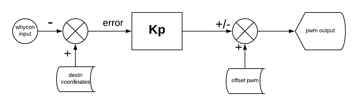
The whycon input consists of x, y and z coordinates which give the current location of the drone. Suppose the destination is say, (x1, y1, z1), then the difference of coordinates, i.e., (x1-x), (y1-y), (z1-z), will be fed as an input to the P-controller. The resultant product, i.e., Kp * error, will be added or subtracted to the offset pwm as the need be to give the final output.

Observations

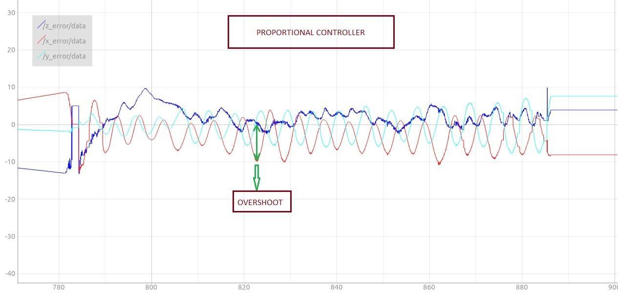
It was observed that the drone never settled at its destination. Instead it oscillated about its destination. The higher the value of Kp the more the amplitude of the oscillation and the drone would be out of the flying zone. Below is a plot between error in x, y, and z coordinates and time. Clearly it is visible that the drone was not able to stabilise itself at the destination.

Hence, it was concluded that a P-controller by itself wasn’t able to stabilise the drone at a required point.

PD Controller

In the previous section we saw how the P-Controller wasn’t successful in stabilising the drone at a given point. It was observed that there were oscillations instead. These oscillations can be damped by using a differential gain along with the P-Controller. The system as a whole is said to be a PD Controller.

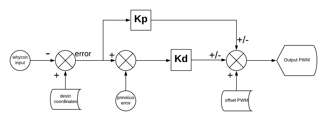
The differential gain Kd is multiplied with the difference of error and previous error. Previous error is a variable that holds the last error generated by the controller output. The controller output in this case is given as:

\text{output} = K_p \cdot \text{error} + K_d \cdot \big( \text{error} - \text{previous error} \big)

Note that Kd is calculated keeping the sampling time in consideration. This output will be further added or subtracted to the offset pwm as the need be to give the final output.

Observations

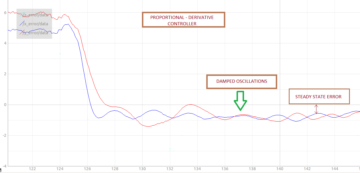
The results of this controller were no match to the P-controller. The oscillations were damped with change in time. Here is a plot of error and time for a PD controller implemented on the Pluto drone.

But, there was a hitch! On having a closer look it was observed that though the drone could hover with respectable stability, it did not do so over the correct point, i.e., the drone did not reach its destination instead it would hover at a point near to the destination. This slight error is known as the steady state error. Hence, it was concluded that a PD controller also by itself wasn’t able to stabilise the drone at the correct destination.

PID Controller

In the previous section we saw how a PD controller was not quite enough. In order to minimise the steady state error we introduce another gain called Ki, the integral gain. Such a system is said to be a PID Controller.

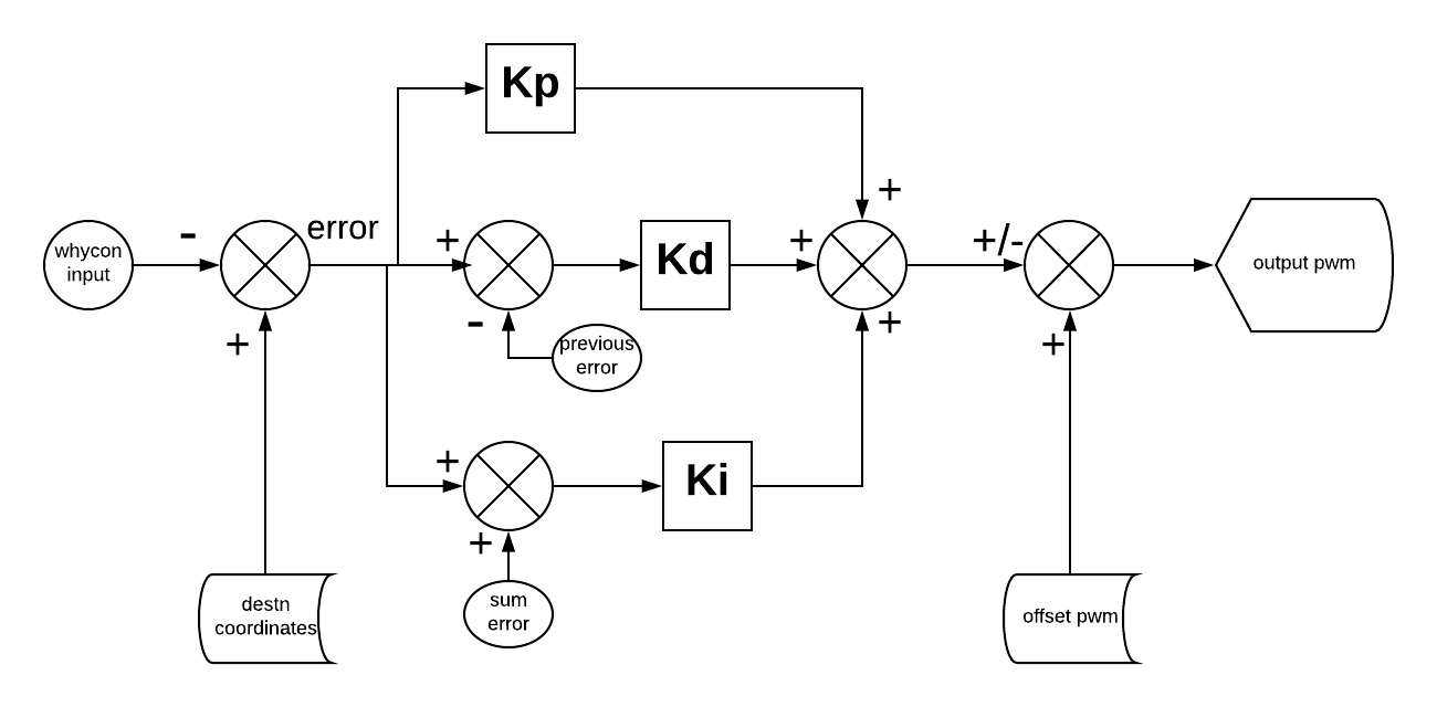
pid_contol_block diagram — Block diagram

Here in we keep track of the error over time i.e. sum up the errors over a specified sampling time.

I_{\text{term}} = \big( I_{\text{term}} + \text{error} \big) \cdot K_i

Further explanation regarding implementation of this Iterm is given in the code. Note that Ki is calculated keeping the sampling time in consideration. This output will be further added or subtracted to the offset pwm as the need be to give the final output.

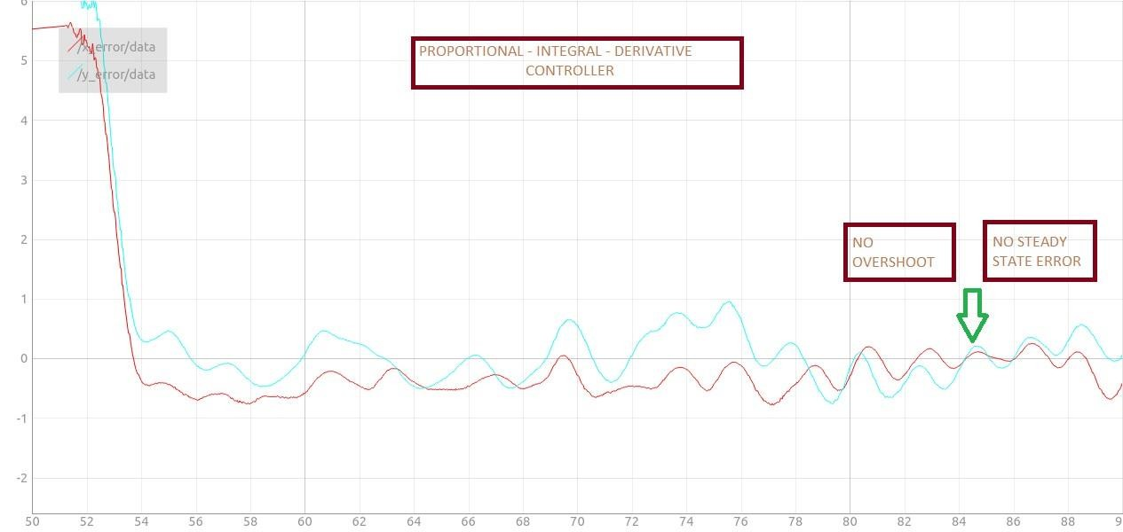
\text{output} = K_p \cdot \text{error} \;+\; I_{\text{term}} \;+\; K_d \cdot \big( \text{error} - \text{previous error} \big)

Observations

The PID controller was successful in hovering the drone above the destination point with minimal error. It overcame the steady state error which was noticeable in previous controllers. Here is a plot of error and time for a PID controller implemented on the Pluto drone.

To sum it up:

Understanding PID Control(by Matlab)

This series provides an introduction to proportional-integral-derivative (PID) control.

PID is just one form of feedback controller, and it can be fairly easy to understand and implement. It is the simplest type of controller that uses the past, present, and future error, and it’s these primary features that you need to satisfy most control problems. That is why PID is the most prevalent form of feedback control for a wide range of real applications..

Often, when learning something new in control theory, it’s easy to get bogged down in the detailed mathematics of the problem. So in this series, we’re going to skip most of the math and instead focus on building a solid foundation..

Throughout this series, you’ll learn what a PID controller is, how to modify it to make it more robust, and you’ll get an overview of tuning methods. Along the way, you’ll understand how PID controllers are used to handle practical applications like actuator saturation and the anti-windup algorithms that protect against it, sensor noise and the derivative filter that is required, and multi-loop control.