Holonomic Drive — Theory & Kinematics

At first glance, the robots of Holonomic Bots look like they’re defying physics — sliding sideways, spinning in place, and gliding diagonally without turning their wheels.
The secret? Omni-wheels.

What is an Omni-Wheel?

An omni-wheel is a special wheel that allows motion in two perpendicular directions:

• Like a normal wheel, it rolls forward and backward.
• Thanks to small rollers mounted around its circumference, it can also slide sideways with minimal resistance.

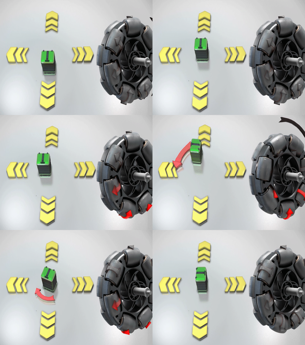
Fig 1: An omni-wheel’s rollers let it roll forward like a normal wheel while sliding freely sideways.

This dual freedom makes omni-wheels the building blocks for holonomic drive systems, where robots can move in any direction without rotating first.

Why Omni-Wheels?

• Conventional wheels restrict motion to only forward/backward (like a car).
• Omni-wheels allow the robot to move laterally, diagonally, or rotate while translating.
• By carefully placing omni-wheels at specific angles (e.g., 120° or 90° apart), the combined forces generate true omnidirectional mobility.

What is a 3-Wheel Holonomic Robot?

A single omni-wheel unlocks two degrees of freedom — but when we combine three omni-wheels in a smart configuration, something magical happens: we get a fully holonomic robot, capable of moving in any direction and rotating, independently and simultaneously.

In Holo Battalion, our robots (Glacio, Crystal, and Frostbite) are equipped with three omni-wheels arranged at 120° intervals:

• Right Wheel ($W_1$)
• Left Wheel ($W_2$)
• Rear Wheel ($W_3$)

This triangular arrangement gives the robot complete control over its motion in the plane.

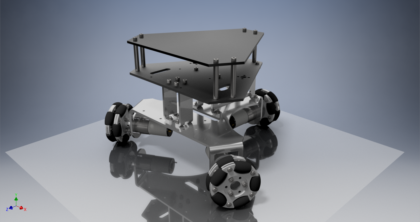
Fig 2: Three omni-wheels ($W_1$, $W_2$, $W_3$) mounted at 120° intervals give the robot full planar mobility.

With this configuration, the robot has 3 controllable motions:

• Forward/Backward ($y$-axis)
• Sideways ($x$-axis)
• Rotation ($\omega$, clockwise positive)

Unlike differential drive robots, the holonomic robot doesn’t need to re-orient before moving sideways or diagonally — it can instantly slide in any direction.

Why 3 Wheels?

• Minimum requirement: To achieve holonomic motion in a plane ($x$, $y$, $\theta$), we need at least 3 actuators.
• Adding more wheels (like 4 or 6) increases stability, but 3 wheels provide a compact and efficient design.
• This configuration balances simplicity, maneuverability, and mathematical elegance for deriving kinematic equations.

Constrained vs. Unconstrained Motion

A constraint on a dynamical system that can be integrated in this way to eliminate one of the variables is called a holonomic constraint. A constraint that cannot be integrated is called a nonholonomic constraint. Constrained and unconstrained motions can provide full omnidirectional motion, or arbitrary translation and rotation when three or more of these wheels are utilized on a platform. The wheels are positioned evenly spaced apart from the platform’s centre, with a consistent separation angle between adjacent pairs of wheels and their driving direction vectors oriented tangentially to the circle that connects them. The three-wheeled design is easy to operate mechanically. The universal wheel’s design makes it possible to achieve a velocity without using any external driving power. The other wheels’ rotation provides the force. The induced velocity is the speed that is created, is shown below.

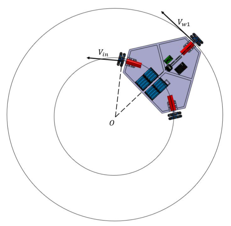
Fig 3: With the left wheel locked, driving the top-right wheel induces a velocity $V_{in}$ perpendicular to the locked wheel’s rolling direction.

The top-right wheel is shown to be moving, but the left wheel is locked and unable to turn around its axle. If there is no slippage, the only way that can roll is perpendicular to the left wheel’s direction of travel. The left wheel, which is not being driven, has since reached velocity $V_{in}$. The induced velocity is as follows. The junction of the lines parallel to $V_{w1}$ and $V_{in}$ marks the location of the platform’s rotational center.

The Math Behind Motion

The three-wheeled holonomic drive system that utilises omni wheels with rollers all around their treads. These wheels can slip laterally as well as drive in the direction of a regular wheel. The control of a three-wheeled holonomic drive robot involves using trigonometry and matrices, as well as understanding forward kinematics and inverse kinematics.

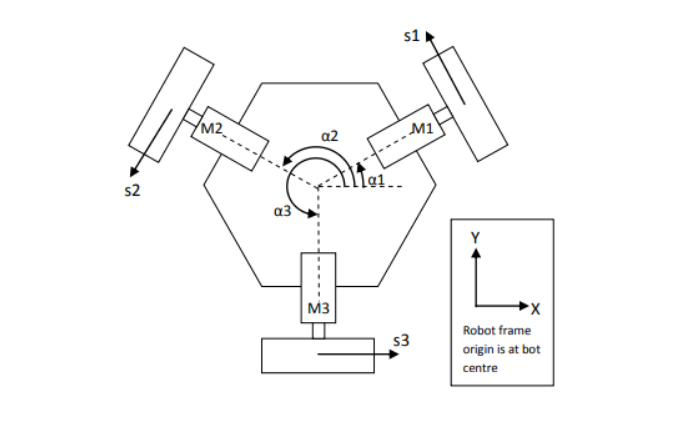
Fig 4: Motor axis angles ($\alpha_1$, $\alpha_2$, $\alpha_3$), measured from the robot’s $x$-axis, used to derive the kinematic equations.

To control a Holonomic Drive robot, you need to consider the orientation of the motor axes and their corresponding angles ($\alpha$) with respect to the x-axis of the robot’s coordinate frame. For example, let’s assume the following values for the motor angles in degrees:

$$\alpha_1 = 30^\circ, \quad \alpha_2 = 150^\circ, \quad \alpha_3 = 270^\circ$$

When the motor turns clockwise (as seen from the wheel end), it will drive the wheel in the direction shown by the ‘s’ arrows. It’s important to note that omni wheels slip in the direction of the motor axis $\alpha$. The wheel drive axis, indicated by the ‘s’ arrow, is oriented at $90^\circ$ or $\pi/2$ from its respective $\alpha$ angle.

To control the robot’s movement, you can utilise forward kinematics to determine the resulting robot velocity based on the wheel velocities. This involves using trigonometric calculations and matrices to translate the wheel velocities into the overall robot velocity.

Inverse kinematics can be used to determine the required wheel velocities based on the desired robot velocity and direction. By applying trigonometry and matrix operations, you can compute the appropriate wheel velocities that will achieve the desired movement.

Understanding these concepts of trigonometry, matrices, forward kinematics, and inverse kinematics is essential in effectively controlling a Holonomic Drive robot.

To control the Holonomic Drive robot and determine its overall motion in the $x$, $y$, and $\omega$ (rotation) directions, you can use the following equations and matrix representation:

Given:

• $\alpha_1 = 30^\circ$, $\alpha_2 = 150^\circ$, $\alpha_3 = 270^\circ$
• Wheel speeds: $s_1$, $s_2$, $s_3$

To calculate the $x$ and $y$ components of the robot’s motion, we resolve the wheel drive orientation vectors’ into $x$ and $y$ components using trigonometry:

For each wheel:

$$x_1 = \cos\left(\alpha_1 + \frac{\pi}{2}\right) s_1, \quad y_1 = \sin\left(\alpha_1 + \frac{\pi}{2}\right) s_1$$ $$x_2 = \cos\left(\alpha_2 + \frac{\pi}{2}\right) s_2, \quad y_2 = \sin\left(\alpha_2 + \frac{\pi}{2}\right) s_2$$ $$x_3 = \cos\left(\alpha_3 + \frac{\pi}{2}\right) s_3, \quad y_3 = \sin\left(\alpha_3 + \frac{\pi}{2}\right) s_3$$

To calculate the overall motion of the robot in the $x$ and $y$ directions, we sum up the contributions from each wheel:

$$x = x_1 + x_2 + x_3$$ $$y = y_1 + y_2 + y_3$$

Substituting the expressions for $x_i$ and $y_i$, we have:

$$x = \cos\left(\alpha_1 + \frac{\pi}{2}\right) s_1 + \cos\left(\alpha_2 + \frac{\pi}{2}\right) s_2 + \cos\left(\alpha_3 + \frac{\pi}{2}\right) s_3$$ $$y = \sin\left(\alpha_1 + \frac{\pi}{2}\right) s_1 + \sin\left(\alpha_2 + \frac{\pi}{2}\right) s_2 + \sin\left(\alpha_3 + \frac{\pi}{2}\right) s_3$$

The rotation of the robot $\omega$ is simply the summation of the wheel speeds:

$$\omega = s_1 + s_2 + s_3$$

We can represent the above equations in matrix form as:

$$\begin{bmatrix} x \\ y \\ \omega \end{bmatrix} = \begin{bmatrix} \cos\left(\alpha_1 + \frac{\pi}{2}\right) & \cos\left(\alpha_2 + \frac{\pi}{2}\right) & \cos\left(\alpha_3 + \frac{\pi}{2}\right) \\ \sin\left(\alpha_1 + \frac{\pi}{2}\right) & \sin\left(\alpha_2 + \frac{\pi}{2}\right) & \sin\left(\alpha_3 + \frac{\pi}{2}\right) \\ 1 & 1 & 1 \end{bmatrix} \begin{bmatrix} s_1 \\ s_2 \\ s_3 \end{bmatrix}$$

Here, the left matrix represents the transformation from the motor speeds ($s_1$, $s_2$, $s_3$) to the resulting motion ($x$, $y$, $\omega$) of the robot.

By solving this matrix equation, you can determine the appropriate motor speeds ($s_1$, $s_2$, $s_3$) required to achieve the desired motion ($x$, $y$, $\omega$) of the robot in its coordinate frame.

The inverse kinematics approach allows us to determine the motor speeds required to send the robot to a desired location in terms of $x$, $y$, and $\omega$, without the need for setting motor speeds $s$ and then calculating the resulting motion. This is in contrast to forward kinematics, where we start with motor speeds and calculate the resulting robot motion.

In inverse kinematics, the first step is to invert the matrix $M$ from the forward kinematics equations. The inverse matrix, denoted as $M^{-1}$, satisfies the equation $M^{-1}M = I$, where $M^{-1}$ is the inverse of $M$ and $I$ is the identity matrix.

By finding the inverse matrix $M^{-1}$, we can solve the equation:

$$\begin{bmatrix} s_1 \\ s_2 \\ s_3 \end{bmatrix} = M^{-1} \begin{bmatrix} x \\ y \\ \omega \end{bmatrix}$$

This allows us to determine the motor speeds $s_1$, $s_2$, and $s_3$ that need to be set in order to send the robot to the desired location and achieve the desired motion in terms of $x$, $y$, and $\omega$.

It’s important to note that calculating the inverse matrix can be complex, especially if the angles $\alpha_1$, $\alpha_2$, and $\alpha_3$ are not orthogonal or if the matrix $M$ is not invertible. In such cases, additional techniques or numerical methods may be necessary to accurately solve for the motor speeds required for the desired robot motion.

Set the body twist ($v_x$, $v_y$, $\omega$) with the sliders and watch the inverse kinematics compute each wheel’s speed live — then hit Drive to see the robot follow that motion.

---