Holonomic Drive — PID Control

Moving the Bot with PID Control

Imagine telling one of our Holo Battalion robots:

Go stand exactly at that spot over there and rotate 630° clockwise!

Sounds simple to us humans. But for a robot, it’s tricky—because it has no intuition about how to correct its own mistakes.

That’s where a PID Controller (Proportional–Integral–Derivative) comes in. It’s like giving the robot a sense of correction:

• If it’s too far from the goal, move harder.
• If it’s close, slow down.
• If it keeps missing the target, remember past mistakes and adjust.
• If it’s heading in the wrong direction, correct proactively.

This loop of measure → compare → correct → repeat is what makes robots move precisely from Point A to Point B.

The Control Loop

1. Feedback: The overhead camera with ArUco markers gives the robot its current pose:

   $$(x, y, \theta)$$

2. Setpoint: This is the desired pose (the goal point you want the robot to reach).

3. Error: The difference between the setpoint and the feedback:

   $$e_x = x_{goal} - x_{current}, \quad e_y = y_{goal} - y_{current}, \quad e_\theta = \theta_{goal} - \theta_{current}$$

4. Controller Action: The PID controller takes this error and decides the velocity commands:

   $$(v_x, v_y, \omega)$$

   These velocities are then converted to wheel speeds via inverse kinematics.

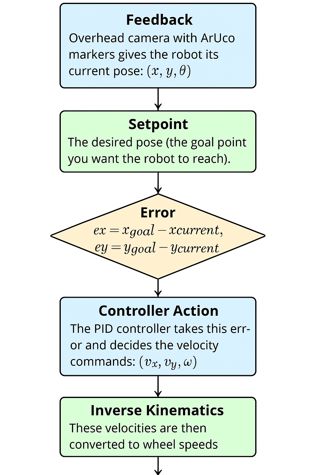
Fig 1: The PID control loop — feedback, setpoint, error, and controller action driving the robot’s velocity commands.

The PID Equation

For one control variable (say $e_x$), the PID controller computes:

$$u(t) = K_p \cdot e(t) + K_i \int e(t)\, dt + K_d \cdot \frac{de(t)}{dt}$$

Where:

• $K_p$: Proportional gain — reacts to how big the error is right now.
• $K_i$: Integral gain — accounts for accumulated error over time (good for biases/drift).
• $K_d$: Derivative gain — predicts future error by looking at the rate of change (helps smooth movement).

Intuitive Analogy

Imagine driving a car to stop at a traffic light:

• Proportional: The harder you press the brake depends on how far you are from the stop line.
• Integral: If you keep overshooting every time, you learn to start braking earlier (memory of past mistakes).
• Derivative: If you’re rushing fast toward the stop line, you slam the brake harder (anticipation of future error).

The balance of these three is what makes a smooth stop.

Implementing PID for the Robot

1. Compute the errors:

   • $e_x = x_{goal} - x_{current}$
   • $e_y = y_{goal} - y_{current}$
   • $e_\theta = \theta_{goal} - \theta_{current}$

2. Run a separate PID loop for each:

   • One PID for $v_x$ (sideways).
   • One PID for $v_y$ (forward/backward).
   • One PID for $\omega$ (rotation).

3. Update at each control cycle (~20–40 Hz).

4. Convert ($v_x$, $v_y$, $\omega$) into wheel velocities using your inverse kinematics equations.

PID Gains and Tuning

• $K_p$: Too low → robot moves sluggishly. Too high → robot overshoots and oscillates.
• $K_i$: Fixes steady-state error (e.g., camera offset or wheel slip). Too high → robot keeps “integrating” and overshoots badly.
• $K_d$: Helps damp oscillations. Too high → robot becomes jittery.

Start simple:

• Begin with only $K_p$.
• Increase until the robot responds but doesn’t oscillate wildly.
• Add a small $K_d$ to smooth motion.
• Finally, add $K_i$ to fix any drift/offset.

In practice, you’ll write something like:

# Pseudocode for PID loop
error = setpoint - measurement
integral += error * dt
derivative = (error - prev_error) / dt

output = Kp * error + Ki * integral + Kd * derivative

prev_error = error

And repeat this for ($x$, $y$, $\theta$).

By combining PID controllers with your inverse kinematics, your holonomic bot can glide precisely to any point in the warehouse floor, using just its ArUco feedback.

---

References

---