Introduction to Coordinate Transform

At first glance, robots moving on the ground or in the air might seem almost magical — turning, sliding, or spinning effortlessly as if they had a mind of their own. How do engineers make this possible? The secret lies in coordinate transformations — the mathematical framework that allows us to describe and control every movement of a robot in space. In this tutorial, we’ll break down these concepts step by step. So, let’s start with:

Representing a Robot in Space

The first step in describing a robot’s motion mathematically is deciding how we represent the robot itself. The simplest approach is to use a single point. Moving this point shows where the robot is, but it has limitations: it can’t show rotation, shape, or size.

To capture more details, we can represent the robot using multiple points. This could be as simple as a triangle or rectangle, or as detailed as a full CAD model, depending on what we need. By placing these points in different positions and orientations, we get a better idea of how the robot moves in space.

Figure 1: A simple 2D representation of three robots using multiple points. Each point marks a corner or reference location, allowing us to visualize the robot's position and shape in space.

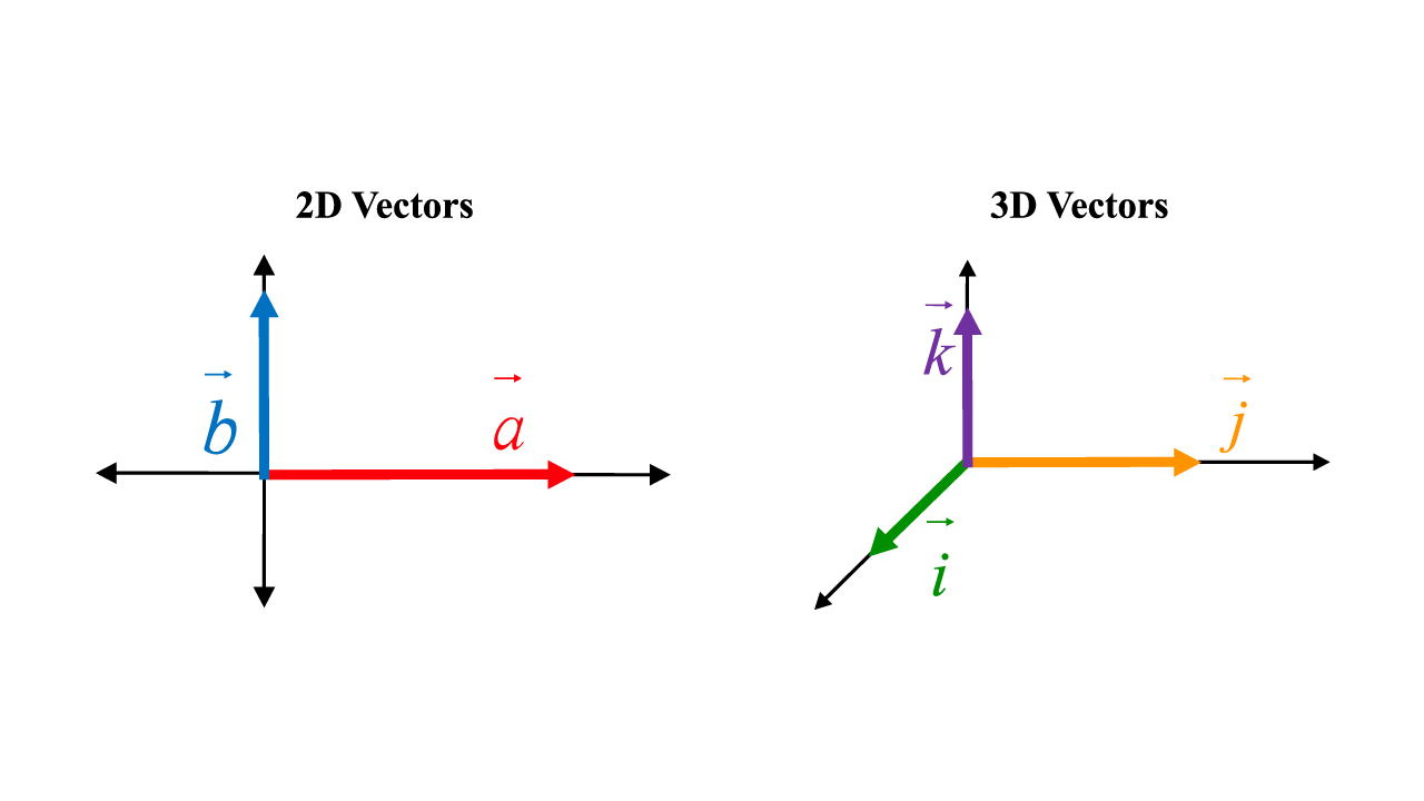
Representing Robots with Points and Vectors

For many robots, movement is limited to a flat surface, like the ground. In such cases, a 2D representation is sufficient and easier to work with. For flying drones or robots moving freely in space, a 3D representation is necessary.

We’ll start by describing robots as a set of points moving in space, which can also be interpreted as vectors representing their position relative to a reference point. Later, we’ll see how multiple coordinate systems, also called reference frames, make calculations easier for more complex robots.

Each point isn’t just a dot on the map — think of it as a position vector from the origin, like a tiny soldier reporting its location to headquarters. This is how we’ll move and rotate our robots precisely. (Don’t worry — we’ll dive into the transformations a bit later, so hold your formation!)

A point (or position vector) in 2D is represented as:

$$\mathbf{p}_{2D} = \begin{bmatrix} x \\ y \end{bmatrix}$$

A point (or position vector) in 3D is represented as:

$$\mathbf{p}_{3D} = \begin{bmatrix} x \\ y \\ z \end{bmatrix}$$

While other systems like polar coordinates exist, Cartesian coordinates ($x$, $y$, $z$) are most common for robotics.

Figure 2: Representation of robots as vectors in 2D and 3D space. Each arrow shows the position of a robot relative to the origin, illustrating how vectors describe location in different dimensions.

Introduction to Coordinate Frames

So far, we’ve represented a robot’s position using points or vectors relative to a single reference point (the origin). In simple scenarios, this works well, but many robots operate in more complex environments where multiple reference points are useful.

A coordinate frame (or reference frame) is essentially a set of axes attached to a specific location and orientation. It allows us to describe the position and orientation of objects relative to that frame instead of just the global origin.

Example:

• The robot’s own frame moves with it, making it easy to describe movements relative to the robot.

• The world frame is fixed to the environment, describing positions in a global context.

Using multiple coordinate frames simplifies calculations, especially when dealing with moving robots, robotic arms, or drones, because we can transform positions and orientations between different frames instead of recalculating everything from scratch.

Different Types of Coordinate Systems

Coordinate frames can be represented in different coordinate systems, depending on the application:

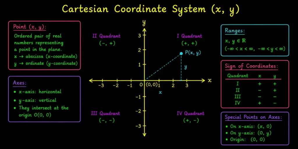
• Cartesian Coordinates ($x$, $y$, $z$)
  • Most common in robotics.
  • Uses perpendicular axes to describe position.

Figure 3: Representation of cartesian coordinate systems.

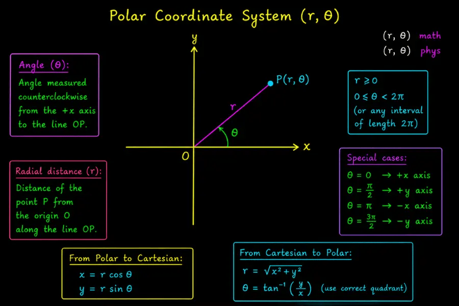
• Polar Coordinates ($r$, $\theta$)
  • Useful for 2D systems with rotational symmetry.
  • Position described by distance and angle from the origin.

Figure 4: Representation of polar coordinate systems.

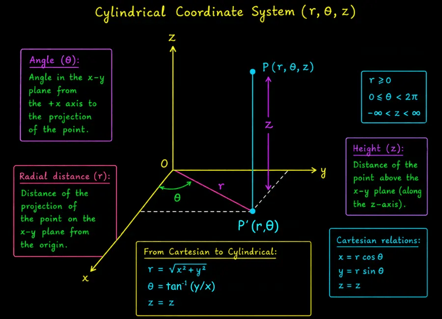
• Cylindrical Coordinates ($r$, $\theta$, $z$)
  • Extension of polar coordinates to 3D.
  • Combines circular motion in the XY-plane with height $z$.

Figure 5: Representation of cylindrical coordinate systems.

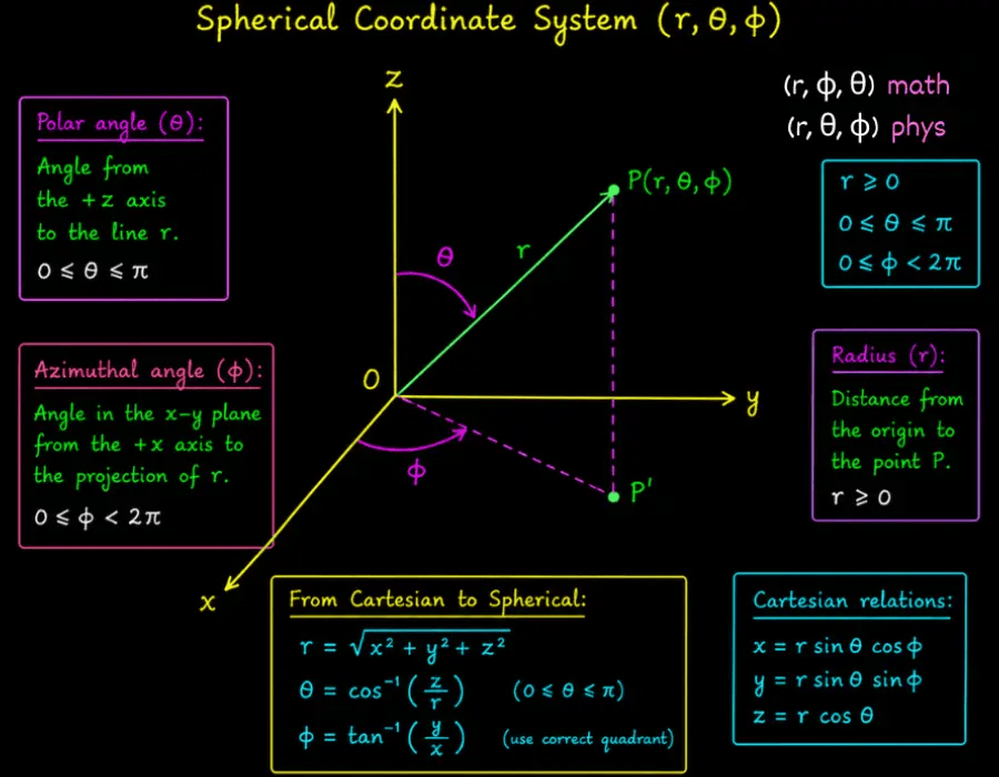
• Spherical Coordinates ($\rho$, $\theta$, $\varphi$)
  • 3D systems where position is described by radius, azimuth angle, and polar angle.
  • Useful for drones, cameras, and robotic arms with rotational joints.

Figure 6: Representation of spherical coordinate systems.

By choosing the right coordinate system, we can simplify calculations and better match the robot’s motion to the task.

Transformations: Moving Robots in Space

A transformation is a mathematical operation that changes a point or vector from one position, orientation, or scale to another. Transformations allow us to move or rotate the robot’s points while keeping track of their relative positions.

1. Translation

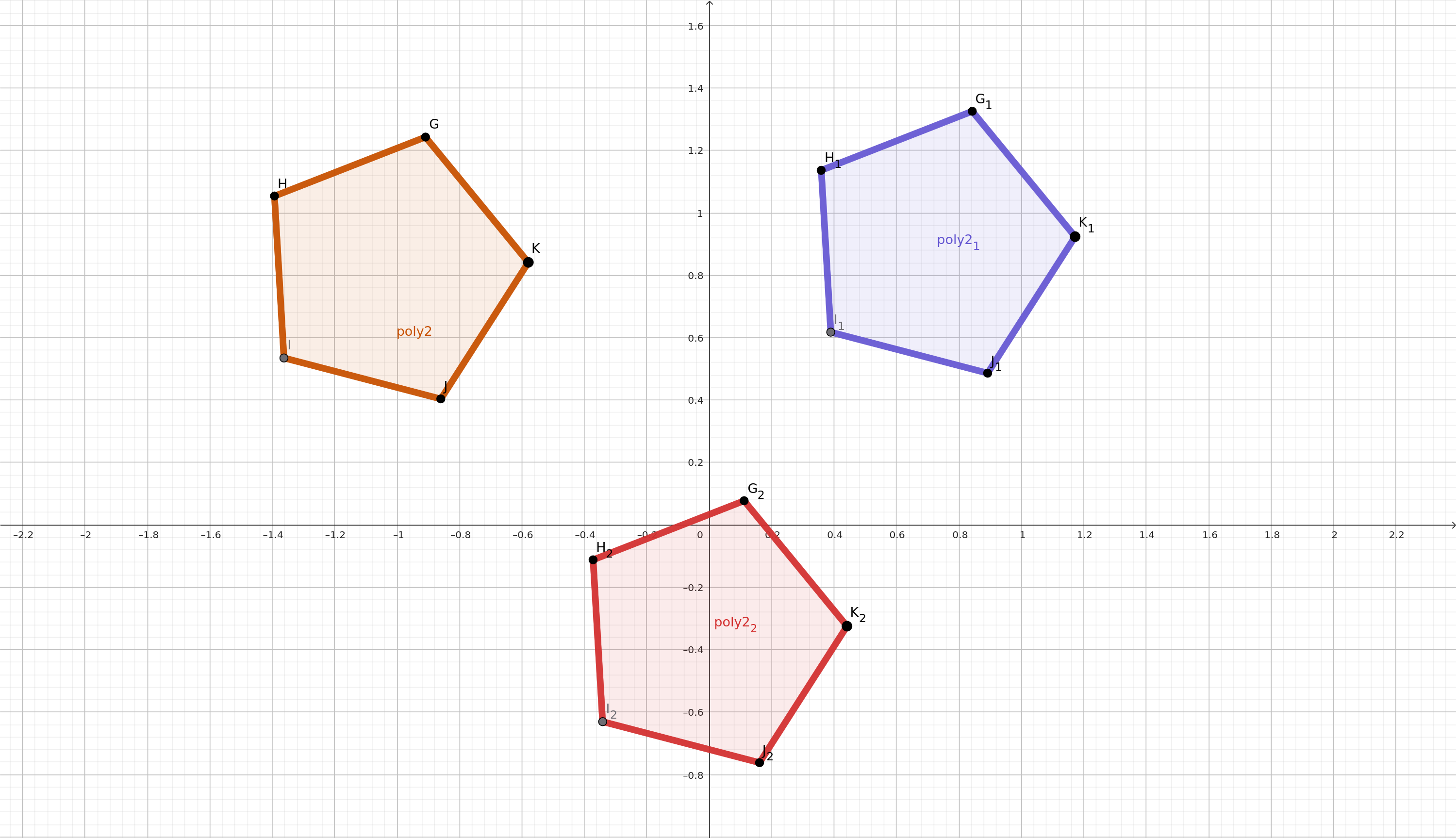
Translation moves points or vectors from one location to another along the X and Y axes.

Here’s the catch: translation can’t be written as a plain matrix multiplied by [x, y]. Any 2×2 matrix always sends the origin (0,0) to itself — that’s just how linear maps work — but translation is supposed to move the origin too. To get around this, we lift the point into one extra dimension by appending a constant 1, called homogeneous coordinates. In this padded form, translation does become an ordinary matrix multiplication, which is why every point below is written as a 3×1 column ending in 1, and every transformation as a 3×3 matrix.

Example:

A point

$$\mathbf{p} = \begin{bmatrix} x \\ y \\ 1 \end{bmatrix}$$

can be translated using a homogeneous transformation matrix:

$$\mathbf{p}' = \begin{bmatrix} x' \\ y' \\ 1 \end{bmatrix} = \begin{bmatrix} 1 & 0 & t_x \\ 0 & 1 & t_y \\ 0 & 0 & 1 \end{bmatrix} \begin{bmatrix} x \\ y \\ 1 \end{bmatrix} = \begin{bmatrix} x + t_x \\ y + t_y \\ 1 \end{bmatrix}$$

Where:

• $x'$, $y'$ are the new coordinates of the point after translation.
• $t_x$, $t_y$ are the translation distances along the X and Y axes.

Tip: You can imagine this as sliding the point along the plane without rotating it.

Try translating the robot by moving the slider!

2. Rotation

Rotation rotates points around the origin (or another point).

Example:

The 2D rotation of a point can be represented by the rotation matrix:

$$R(\theta) = \begin{bmatrix} \cos\theta & -\sin\theta \\ \sin\theta & \cos\theta \end{bmatrix}$$

Where:

• $\theta$ is the rotation angle in radians.
• Multiplying this matrix by a column vector $\mathbf{p} = \begin{bmatrix} x \\ y \end{bmatrix}$ rotates the point by $\theta$.

Rotation is a linear operation — it fixes the origin — so it doesn’t strictly need the homogeneous trick. But writing it in the same 3×3 form as translation is what lets the two be combined later into a single matrix:

$$R(\theta) = \begin{bmatrix} \cos\theta & -\sin\theta & 0 \\ \sin\theta & \cos\theta & 0 \\ 0 & 0 & 1 \end{bmatrix}$$

Try moving the slider to rotate the robot!

3. Scaling

Scaling changes the size of the shape relative to a point (usually the origin).

Example:

$$\mathbf{p}' = \begin{bmatrix} s_x & 0 \\ 0 & s_y \end{bmatrix} \mathbf{p}$$

Like rotation, scaling already fixes the origin — but again, writing it in homogeneous form keeps it compatible with translation and rotation so all three can be chained together:

$$\begin{bmatrix} s_x & 0 & 0 \\ 0 & s_y & 0 \\ 0 & 0 & 1 \end{bmatrix}$$

Try moving the sliders to scale the robot!

Combining Transformations

In robotics, it is often necessary to apply multiple transformations to a robot or object, such as translation, rotation, and scaling. Because each transformation is now a matrix, combining them is just matrix multiplication — but the order of transformations matters:

• Rotate → Translate is different from Translate → Rotate.
• Understanding this order is crucial to position and orient robots correctly.

Note on order: a matrix acts on whatever sits immediately to its right. So in a product like $R \cdot T \cdot \mathbf{p}$, T is applied to the point first and R second — the order you read the matrices in is the reverse of the order the motions actually happen in. Swap the order of multiplication (T · R instead of R · T) and you generally land on a different final position, which is exactly why order matters.

Examples of Combined Transformations

1. Translation + Rotation

$$\begin{bmatrix} \cos \theta & -\sin \theta & t_x \\ \sin \theta & \cos \theta & t_y \\ 0 & 0 & 1 \end{bmatrix}$$

2. Scaling + Rotation

$$\begin{bmatrix} s_x\cos \theta & -s_y\sin \theta & 0 \\ s_x\sin \theta & s_y\cos \theta & 0 \\ 0 & 0 & 1 \end{bmatrix}$$

3. Full Affine Transformation

Chaining scaling, rotation, and translation together gives the general form that any rigid or affine motion in 2D can be written as:

$$\begin{bmatrix} s_x\cos \theta & -s_y\sin \theta & t_x \\ s_x\sin \theta & s_y\cos \theta & t_y \\ 0 & 0 & 1 \end{bmatrix}$$

Where:

• $x'$, $y'$ are the transformed coordinates
• $\theta$ is the rotation angle
• $t_x$, $t_y$ are translation amounts in the X and Y directions
• $s_x$, $s_y$ are the scale factors along the X and Y directions

This is the same machinery behind the coordinate frames from earlier: if you know a robot’s pose (position + orientation) within its own frame, and the transform that places that frame inside the world frame, multiplying the two — in the right order — gives the robot’s pose in world coordinates. It’s the exact same combined matrix above, just reused to relate two frames instead of two poses of one point.

Try moving the sliders to translate, rotate, and scale the robot together!

Note: This is just an overview of coordinate transformations for robots. To gain a deeper understanding, it is recommended to study linear algebra, which is a fundamental prerequisite for robotics.

---

References

• Essence of Linear Algebra by 3Blue1Brown
• Coordinate Transforms For Robotics by Articulated Robotics

---